CLUSTAG: Hierarchical Clustering and Graph Methods for Selecting Tag SNPs

S. I. Ao^1*, Kevin Yip², Michael Ng¹, David Cheung², Pui-Yee Fong³, Ian Melhado³, Pak C. Sham³

(1) Department of Mathematics, The Univeristy of Hong Kong
(2) Department of Computer Science, The University of Hong Kong
(3) Genome Research Center, The University of Hong Kong

Cluster and set-cover algorithms are developed to obtain a set of tag SNPs that can represent all the known SNPs in a chromosomal region, subject to the constraint that all SNPs must have a squared correlation R² > C with at least one tag SNP, where C is specified by the user. The program is implemented with Java, and it can run in Windows platform as well as the Unix environment.

• How does the hierarchical clustering works for the SNPs
• Graph formulation
• Experimental results
• Download the program
• How to use it
• Acknowledgements
• References
• Supplementary information

How does the hierarchical clustering works for the SNPs

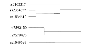
Hierarchical clustering starts with a square matrix of pair-wise distances between the objects to be clustered. For the problem of tag SNP selection, the objects to be clustered are the SNPs, and an appropriate measure of distance is 1-R², where R² is the squared correlation between two SNPs. The rationale is this: the required sample size for a tag SNP to detect an indirect association with a disease is inversely proportional to the R² between the tag SNP and the causal SNP. In agglomerative clustering, the two clusters with the smallest inter-cluster distance are successively merged until all the objects have been merged into a single cluster. Different forms of agglomerative clustering differ in the definition of the distance between two clusters, each of which may contain more than one object. In single-linkage or nearest-neighbour clustering, the distance between two clusters is the distance between the nearest pair of objects, one from each cluster. In complete linkage or farthest neighbour clustering, the distance between two clusters is the distance between the farthest pair of objects, one from each cluster. The clustering process can be represented by a dendrogram, which is a tree diagram showing how the individual objects are successively merged at greater distances into larger and fewer clusters. The user defines a cutoff merging distance, and considers all the distinct clusters that have been generated at that distance or lower (see Figure 1). 

A desirable property for a clustering algorithm, in the context of tag SNP selection, would be that a cluster must contain at least one SNP (the tag SNP) that is no more than the merging distance from all the other SNPs from the same cluster. If this is the case, then by setting a cutoff merging distance of C, one can ensure that no SNP is further than C away from the tag SNP in its cluster. In this sense, neither of the methods proposed by Byng et al (2003) is ideal, since the single-linkage method does not guarantee the existence of a tag SNP with distance less than C from all SNPs in the same cluster, while complete-linkage is too conservative in that all SNPs have distance under C from all other SNPs in the same cluster.

Minimax clustering

In order to achieve the desired property described above, we propose a new definition of the distance between two clusters that, as follows:

* For each SNP belonging to either cluster, find the maximum distance between it and all the other SNPs in the two clusters

* The smallest of these maximum distances is defined as the distance between the two clusters.

*  The corresponding SNP is defined as the tag SNP of the newly merged cluster

We call this method minimax clustering. Similar algorithms have been described for the selection of compounds with diverse properties (Snarey et al, 1997). There is a parrallel in topology in which the distance between two compact sets can be measured by a sup-inf metric known as Hausdorff distance (Barnsley, 1988).

Graph formulation

For comparison we have also implemented an algorithm based on the NP-complete minimum dominating set of the set-cover problem, similar to the greedy algorithm developed by Carlson et al (2004). The set of SNPs are the nodes of a graph, which are connected by edges where their corresponding SNPs have R² > C. The objective is to find a subset of nodes such that that all nodes are connected directly to at least one SNP of that subset. The algorithm is heuristic, and the details can be found in Reuven & Zehavit (2004). Briefly, at the beginning, all the SNPs belong to the untagged set. The algorithm picks the node with the largest number of nodes that are connected directly to this node (without passing through any other nodes) from the untagged set. Then the SNPs inside the selected subset are deleted from the untagged set, and the next largest connected subset is chosen from the untagged set. The algorithm terminates when the untagged set becomes empty.

Experimental results

We have compared the performance of the three implemented algorithms, using SNP data from the ENCODE regions of the HapMap project, according to three criteria: (1) compression, the ratio of clusters to SNPs, (2) compactness, the average distance between a SNP and the tag SNP of its cluster, and (3) run time. Our results show that the compression ratio is roughly equivalent for the set cover and minimax clustering algorithms but substantially higher for the complete linkage (Table 1). The minimax algorithm produces more compact clusters than the set cover algorithm, but takes approximately twice the running time. Further evaluations of these and other algorithms for tag SNP selection are needed.

Fig. 1. Sample illustrative dendrogram showing how 7 SNPs are merged into 3 clusters at or below the cutoff merging distance.

Table 1.  Properties of three tag SNP selection algorithms, evaluated for ENCODE regions.